Code
#### Load libraries
library(ggplot2)
library(tidyverse)
library(ggtext)
library(scales)
library(hrbrthemes)
library(maps)
library(janitor)
library(showtext)
library(MetBrewer)
library(scico)
library(patchwork)
library(gghighlight)
When we think about seafood, we think delicious lobster, shrimp, mussels and tuna. Our senses can be positive and negative, like thinking about how fresh it can be and how maybe not so good it can smell. Maybe we also think about the cost, we all know a really good sushi restaurant comes at a price. But what if you look a little deeper? Look past the seafood itself, and look more closely at the big, often diesel powered, machines used to catch them. The smoke, oil, air pollution, greenhouse gasses are all a byproduct of ocean fishing. This makes you quickly realize the environmental implications of such a massive operation. When you think about the shear number of vessels, quantifying this pollution seems almost impossible. However, with new advancement in Automated Identification System (AIS) tracking and satellite data, this challenge has become more manageable.
The novel dataset has been provided by emLab and Global Fishing Watch. This new data set has geographical locations for every single AIS fishing vessel in the world as well as vessels that are known as the dark fleet, meaning they do not have AIS and do not broadcast a location. With this dataset not only can we can get an idea of the total CO2 pollution associated with global fisheries, but we can also see which countries standout as the biggest contributors. These are important first steps if we want to curb emissions associated with seafood production.
There are some important questions that I wanted to address when making this info graphic:
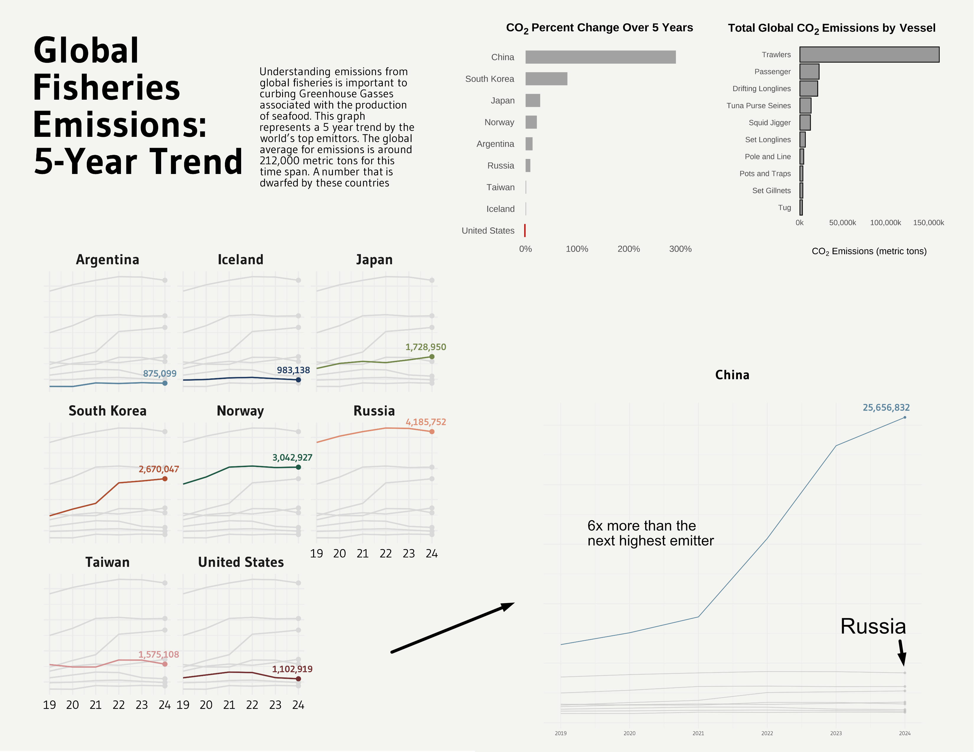
The typography I wanted to keep simple. Text is bold where needed to tell the user, “Hey, there is some important context here!”. For example, it was important that I gave context to just how much more China fishing industry is contributing when compared to the top 10 polluters. I used some bold text within the graph to draw attention to what you are actually looking at. The general design I want to be linearly, meaning it flows well and does not require a complex path on paper. I chose to go wide instead of long because it feels more natural to how someone would read a book. Starting at the top left the reader quickly picks up on the context for the viz and its central message, which is clearly stated immediately in both the title and subtitle.
I want to acknowledge that in today’s climate, DEI is more important than ever. While I think that some emissions can be related to countries who have less resources to invest in more modern equipment, my dataset does not allow me to explore that question.
Accessibility was important to me when making the graphics. I used the {gghighight} package to make data standout for the reader. The colors matter less and act as a contrast to the background. I did create the final plot in Affinity and added alt text in this quarto doc to make this information more available to everyone.
#### Load libraries
library(ggplot2)
library(tidyverse)
library(ggtext)
library(scales)
library(hrbrthemes)
library(maps)
library(janitor)
library(showtext)
library(MetBrewer)
library(scico)
library(patchwork)
library(gghighlight)# read in the data
emissions_years <- read_csv("data/meds_high_resolution_annual_ais_emissions_spatial_data_v20241121.csv")
# group by flag, year and summarize emissions
emissions_by_year <- emissions_years %>%
group_by(flag, year) %>%
summarise(total_co2_mt = sum(emissions_co2_mt)) %>%
ungroup() %>%
mutate(global_avg_co2_mt = mean(total_co2_mt)) %>%
filter(flag %in% top_9$flag,
flag != "CHN")
# gave the countries actual names
emissions_by_year <- emissions_by_year %>%
mutate(flag = recode(flag,
'ARG' = 'Argentina',
'ISL' = 'Iceland',
'JPN' = 'Japan',
'KOR' = 'South Korea',
'NOR' = 'Norway',
'RUS' = 'Russia',
'TWN' = 'Taiwan',
'USA' = 'United States'))
#### MISC ####
font <- "Gudea"
font_add_google(family=font, font, db_cache = TRUE)
fa_path <- systemfonts::font_info(family = "Font Awesome 6 Brands")[["path"]]
font_add(family = "fa-brands", regular = fa_path)
theme_set(theme_minimal(base_family = font, base_size = 10))
bg <- "#F4F5F1"
txt_col <- "black"
showtext_auto(enable = TRUE)
p_1 <- emissions_by_year %>%
ggplot() +
geom_point(data=emissions_by_year %>%
slice_max(year),
aes(x=year, y=total_co2_mt, color=flag),shape=16) +
geom_line(aes(x=year, y=total_co2_mt, color=flag)) +
gghighlight(use_direct_label = FALSE,
unhighlighted_params = list(colour = alpha("grey85", 1))) +
geom_text(data=emissions_by_year %>%
slice_max(year),
aes(x=year, y=total_co2_mt, color=flag, label = scales::comma(round(total_co2_mt))),
hjust = .65, vjust = -1, size=2.5, family=font, fontface="bold") +
scale_color_met_d(name="Redon") +
scale_y_continuous(labels = c("","","","","")
) +
scale_x_continuous(labels = function(x) substring(x, 3, 4)) +
#facet_wrap(~ country) +
facet_wrap(~ factor(flag, levels=c('Argentina','Iceland','Japan', 'South Korea','Norway', 'Russia', 'Taiwan', 'United States'))) +
coord_cartesian(clip = "off") +
theme(
axis.title = element_blank(),
axis.text = element_text(color=txt_col, size=9),
strip.text.x = element_text(face="bold", size = 11),
plot.title = element_markdown(hjust=.5,
size=34,
color=txt_col,
lineheight=.8,
face="bold", margin=margin(20,0,30,0)),
plot.subtitle = element_markdown(hjust=.5,
size=18,
color=txt_col,
lineheight = 1,
margin=margin(10,0,30,0)),
plot.caption = element_markdown(hjust=.5,
margin=margin(60,0,0,0),
size=8, color=txt_col,
lineheight = 1.2),
plot.caption.position = "plot",
plot.background = element_rect(color=bg, fill=bg),
plot.margin = margin(10,10,10,10),
legend.position = "none",
legend.title = element_text(face="bold")
)
text <- tibble(
x = 0, y = 0,
label = "Understanding emissions from global fisheries is important to curbing Greenhouse Gasses associated with the production of seafood. This graph represents a 5 year trend by the world's top emittors. The global average for emissions is around 212,000 metric tons for this time span. A number that is dwarfed by these countries"
)
sub <- ggplot(text, aes(x = x, y = y)) +
geom_textbox(
aes(label = label),
box.color = bg, fill=bg, width = unit(9, "lines"),
family=font, size = 3, lineheight = 1
) +
coord_cartesian(expand = FALSE, clip = "off") +
theme_void() +
theme(plot.background = element_rect(color=bg, fill=bg))
# TITLE
text2 <- tibble(
x = 0, y = 0,
label = "**Global Fisheries Emissions: 5-Year Trend**<br>"
)
title <- ggplot(text2, aes(x = x, y = y)) +
geom_textbox(
aes(label = label),
box.color = bg, fill=bg, width = unit(12, "lines"),
family=font, size = 10, lineheight = 1
) +
coord_cartesian(expand = FALSE, clip = "off") +
theme_void() +
theme(plot.background = element_rect(color=bg, fill=bg))
finalPlot <- ((title+sub)/p_1) +
plot_layout(heights = c(1, 2)) +
plot_annotation(
theme=theme(plot.caption = element_markdown(hjust=0,
margin=margin(0,0,0,0),
size=6, color=txt_col,
lineheight = 1.2),
plot.margin = margin(20,20,20,20),))
print(finalPlot)
showtext_opts(dpi = 600)
# Save the figure
ggsave("Global_fisheries.png",
bg=bg,
height = 8,
width = 5,
dpi = 600)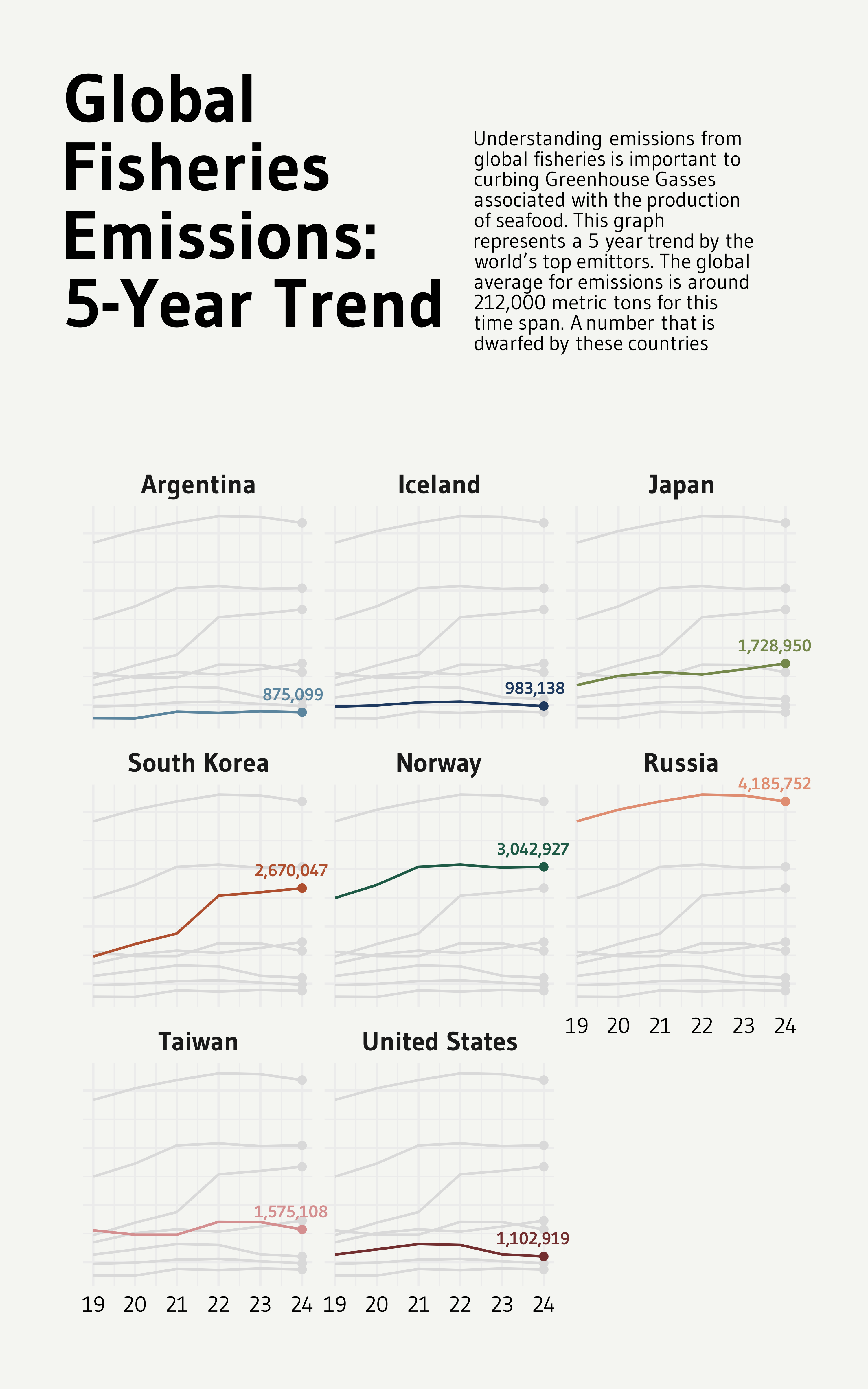 #### Plot 2
# filter for just CO2 for China over the same years
china_emissions <- emissions_years %>%
  group_by(flag, year) %>%
  summarise(total_co2_mt = sum(emissions_co2_mt)) %>%
  ungroup() %>%
  mutate(global_avg_co2_mt = mean(total_co2_mt)) %>%
  filter(flag %in% top_9$flag)

p_4 <- china_emissions %>%
  ggplot()  +
  geom_point(data=china_emissions %>%
               slice_max(year),
             aes(x=year, y=total_co2_mt, color=flag),shape=16) +
  geom_line(aes(x=year, y=total_co2_mt, color=flag)) +
  gghighlight(flag == "CHN",
              use_direct_label = FALSE) +
  geom_text(data=china_emissions %>%
              filter(flag == "CHN") %>%
              slice_max(year),
             aes(x=year, y=total_co2_mt, color=flag, label = scales::comma(round(total_co2_mt))),
             hjust = .90, vjust = -1, size=5, family=font, fontface="bold") +
  scale_color_met_d(name="Redon") +
  labs(title = "China") +
  theme(
    legend.position = "none",
    axis.text.y = element_blank(),
    axis.title.y = element_blank(),
    axis.title.x = element_blank(),
    plot.title = element_markdown(hjust=.5,
                                  size=20,
                                  color=txt_col,
                                  lineheight=.8,
                                  face="bold", margin=margin(20,0,30,0))
        )

print(p_4)

showtext_opts(dpi = 600)

# Save the figure
ggsave("China_fisheries.png",
      bg=bg,
      height = 8,
      width = 8,
      dpi = 600)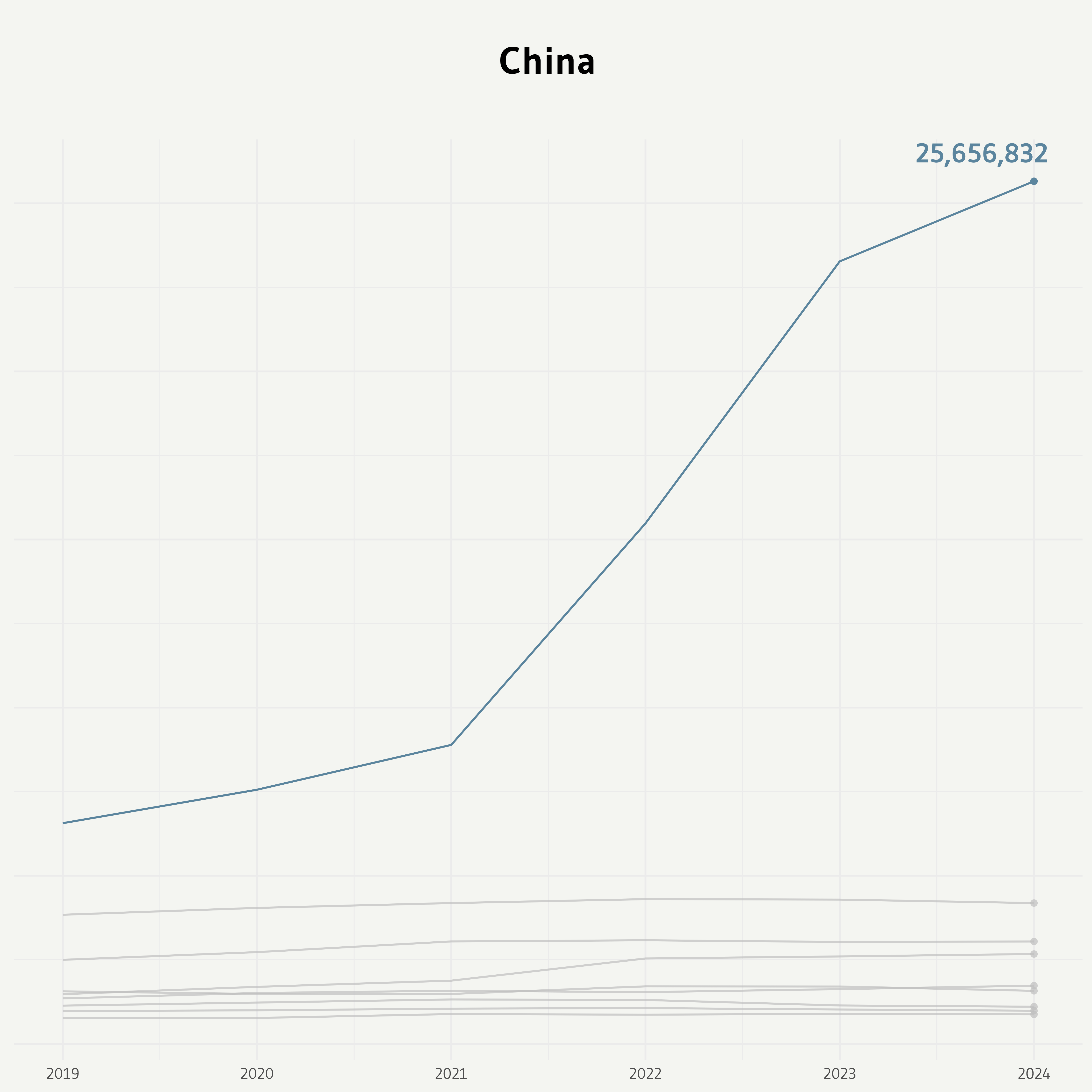
# calculate total emissions over the 5 year span by country
total_19_24 <- china_emissions %>%
filter(year == c(2019, 2024)) %>%
mutate(flag = recode(flag,
'ARG' = 'Argentina',
'ISL' = 'Iceland',
'JPN' = 'Japan',
'KOR' = 'South Korea',
'NOR' = 'Norway',
'RUS' = 'Russia',
'TWN' = 'Taiwan',
'USA' = 'United States',
'CHN' = 'China'))
total_emissions <- total_19_24 %>%
group_by(flag) %>% # Group by the identifier (e.g., country or flag)
mutate(percent_chng = ifelse(year == 2024,
(total_co2_mt - total_co2_mt[year == 2019]) / total_co2_mt[year == 2019] * 100,
NA)) %>%
drop_na() %>%
ungroup()
# Add a column with your condition for the color
total_emissions <- total_emissions %>%
mutate(mycolor = ifelse(percent_chng>0, "type1", "type2"))
# Arrange data in ascending order of percent_chng
total_emissions <- total_emissions %>%
arrange(percent_chng) # Use ascending order
# Set the factor levels for `flag` based on the new order
total_emissions <- total_emissions %>%
mutate(flag = factor(flag, levels = flag)) # Match order to factor levels
# Plot the data
p_2 <- ggplot(total_emissions, aes(x=flag, y=percent_chng)) +
geom_segment(aes(x=flag, xend=flag, y=0, yend=percent_chng, color=mycolor), size=8, alpha=0.9) +
theme_light() +
theme(
legend.position = "none",
panel.border = element_blank(),
axis.text.x = element_text(size = 10),
axis.text.y = element_text(size = 10),
axis.title.x = element_text(size = 5, margin = margin(t = 10)),
plot.title = element_text(size = 14),
plot.background = element_rect(color = bg, fill = bg),
panel.background = element_rect(color = bg, fill = bg)
) +
labs(title = "CO<sub>2</sub> Percent Change Over 5 Years") +
xlab("") +
ylab("Percent Change") +
coord_flip() +
scale_y_continuous(labels = scales::label_percent(scale = 1)) +
scale_color_manual(values = c("type1" = "grey60", "type2" = "#B30600")) +
theme_ipsum() +
theme(plot.title = element_markdown(hjust=.5,
size=15,
color=txt_col,
lineheight=.8,
face="bold"),
axis.title.x = element_blank(),
legend.position = "none",
panel.grid.minor = element_blank(),
panel.grid.major = element_blank())
print(p_2)
showtext_opts(dpi = 600)
# Save the figure
ggsave("total_change_co2.png",
bg=bg,
height = 5,
width = 5,
dpi = 600)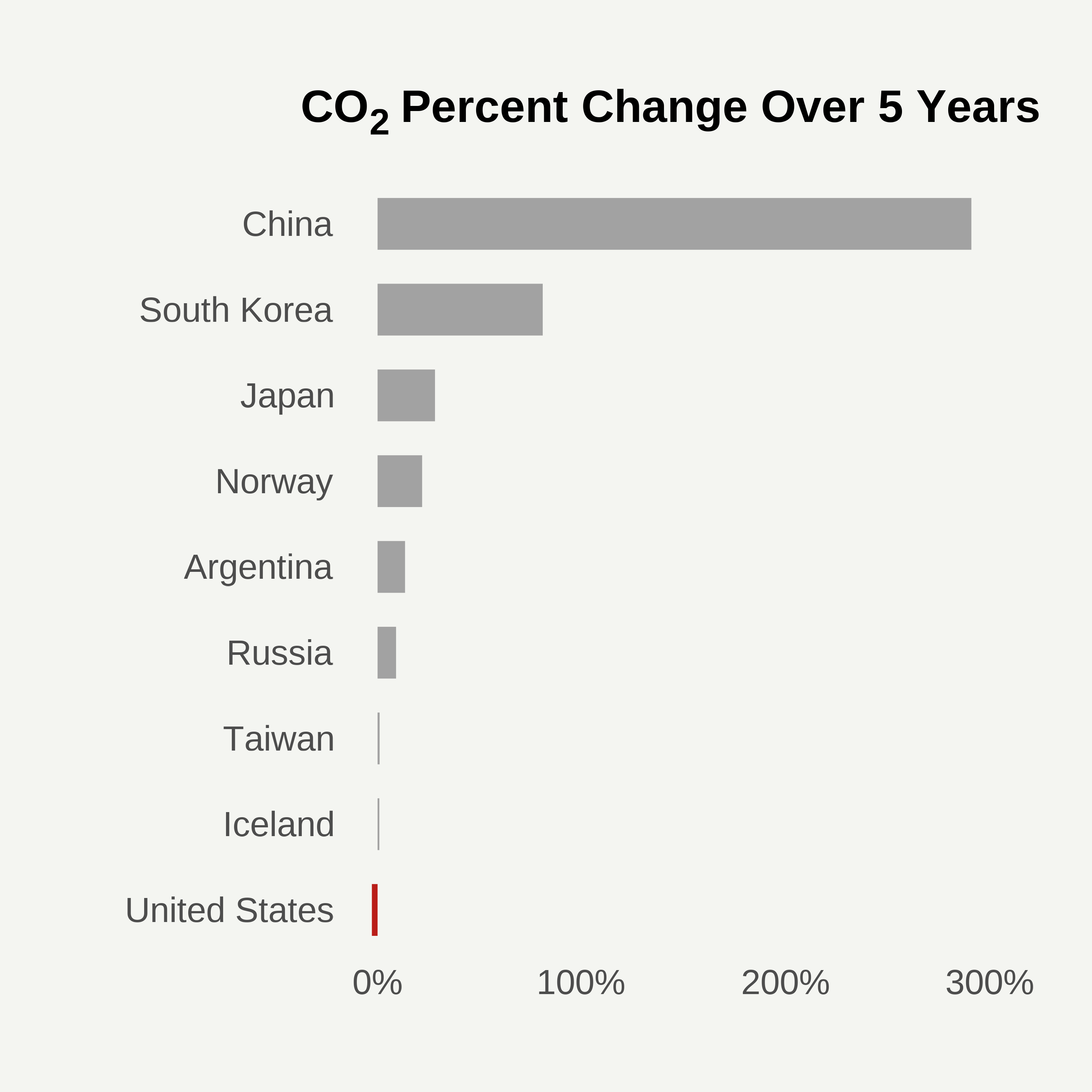 #### Plot 4
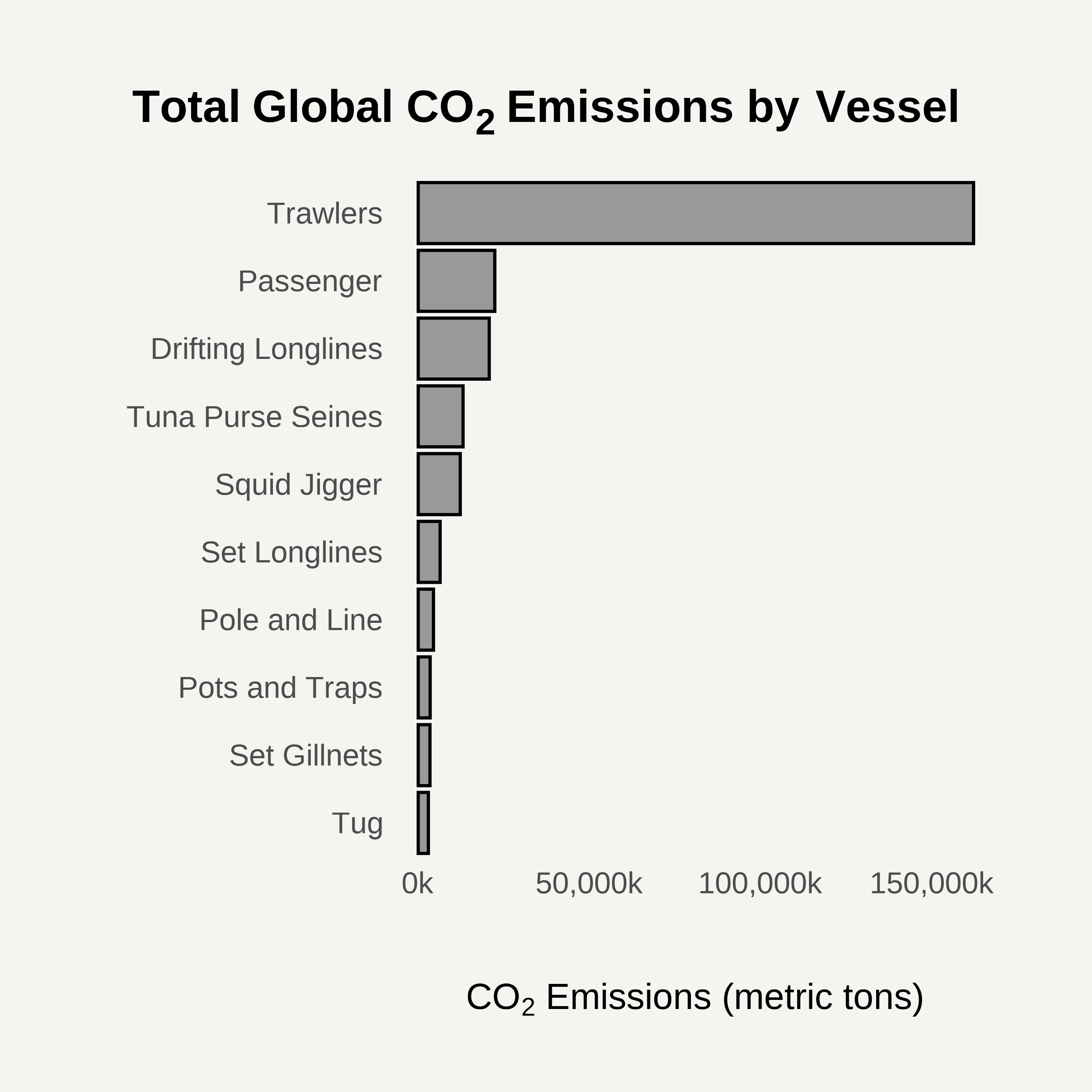
# filter for emissions by vessel type
emission_vessel <- emissions_years %>%
  group_by(vessel_class) %>%
  summarise(total_co2_mt = sum(emissions_co2_mt)) %>%
  arrange(desc(total_co2_mt)) %>%
  slice(1:10)

# rename some of the columns because they are not so pretty to read
emission_vessel <- emission_vessel %>%
  mutate(vessel_class = case_when(
    vessel_class == "trawlers" ~ "Trawlers",
    vessel_class == "squid_jigger" ~ "Squid Jigger",
    vessel_class == "passenger" ~ "Passenger",
    vessel_class == "drifting_longlines" ~ "Drifting Longlines",
    vessel_class == "tuna_purse_seines" ~ "Tuna Purse Seines",
    vessel_class == "pole_and_line" ~ "Pole and Line",
    vessel_class == "set_longlines" ~ "Set Longlines",
    vessel_class == "pots_and_traps" ~ "Pots and Traps",
    vessel_class == "trollers" ~ "Trollers",
    vessel_class == "set_gillnets" ~ "Set Gillnets",
    vessel_class == "other_purse_seines" ~ "Other Purse Seines",
    TRUE ~ vessel_class
  ))

# show the top vessel emitters
p_4 <- ggplot(emission_vessel, aes(vessel_class, y=total_co2_mt, fill=vessel_class)) +
  geom_bar(stat="identity", color="black", fill = "grey60") +
  scale_fill_manual(values=rep("grey", 10)) +
  theme_ipsum() +
  theme(
    legend.position="none",
    plot.title = element_text(hjust=0.5, vjust=1, size=14, margin=margin(b=10)),
    plot.title.position = "plot",
    axis.text.x = element_text(size = 10),
    axis.text.y = element_text(size = 10),
    plot.background = element_rect(color = bg, fill = bg), # Match background
    panel.background = element_rect(color = bg, fill = bg), # Match panel background
    panel.border = element_blank()
  ) +
  xlab("") +
  ylab("") +
  ggtitle("Total Global CO2 Emissions by Vessel") +
  scale_y_continuous(labels = scales::unit_format(unit = "MT", scale = 1e-3)) +
  coord_flip()


showtext_opts(dpi = 600)

# Save the figure
ggsave("total_co2_vessel.png",
      bg=bg,
      height = 5,
      width = 5,
      dpi = 600)